Determining Movie Genre from its Review

Text analysis is a continously growing application of data science that has many practical applications. At SMG we used data science to enhance many of our text analytic services we provide for clients. We overhauled our sentiment classification processes, developed highly accurate detectors for significant TA occurances, prototyped trend detectors and forecasting models for text and built tools and processes to extract entity variants from our large datasets of survey comments.

For this exercise let’s understand how much information about a movie genre is captured in review content. The code used to generate the content shown in this post can be found here.

The Stanford IMDB Dataset

The AI lab at Stanford (SAIL) has done a lot cool stuff over the the years and provides a lot of services to the data science community (the GloVe word embeddings data set is just one good example).

For this exercise we are going to use the Large Movie Review Dataset developed and hosted by the Stanford AI group. The dataset consists of 50,000 movie reviews that have been labeled positive and negative. Half of the reviews are labeled positive while half are labeled negative. The data is organized such that half the reviews are in a test folder and half in a training folder (so 12,500 reviews are positive-training, 12,500 are positive-negative, etc…). You can see the associated paper here.

Scraping Genre from IMDB

The Stanford review dataset has very little meta-data about the film being reviewed – the only information provided is a url to the films corresponding IMDB page. Fortunately in most cases that page has the films genre embedded in it. The code snippet below is used to extract the genre(s) of the film from its IMDB page.

        # request the html data
        # need to remove excess url stuff
        response = requests.get(row[1]['url'].split('/usercomments')[0])

        # parse the text
        soup = BeautifulSoup(response.text, 'html.parser')

        # genre data is in the script tag
        scriptrows = soup.find_all('script')
        try:
            # look in the first one
            cand = [r for r in scriptrows if str(r).split('genre')[0] != str(r)][0]    
            try:
                # multiple genres
                genres = ast.literal_eval(str(cand).split('genre')[1].split(']')[0].replace("\n","").replace('": [',"").lstrip().rstrip())
            except SyntaxError:
                # hit an error
                # because only one genre
                genres = (str(cand).split('genre')[1].split(',')[0].replace("\n","").replace('":',"").lstrip().rstrip().replace('"',""))

            # grab the movie title
            movie_title = soup.title.text.replace(' - IMDb', "")

            # record the data
            movie_data.append((row[0], movie_title, genres))
        except:
            # no genres found -- skip this entry
            print "Error with %i" % row[0]

The result is a dataframe indexed to the dataset that contains the title and genres of each reviewed film:

ref	title	genres
0	Futz (1969)	(Comedy)
1	Stanley & Iris (1990)	(Drama, Romance)
2	Stanley & Iris (1990)	(Drama, Romance)
3	Stanley & Iris (1990)	(Drama, Romance)
4	The Mad Magician (1954)	(Horror, Mystery, Thriller)

You can see a couple of attributes stand out about the data. First, there are multiple reviews for the same movie. We can see this if we dig into the data. Here is the review for ref 2:

I saw the capsule comment said “great acting.” In my opinion, these are two great actors giving horrible performances, and with zero chemistry with one another, for a great director in his all-time worst effort. Robert De Niro has to be the most ingenious and insightful illiterate of all time. Jane Fonda’s performance uncomfortably drifts all over the map as she clearly has no handle on this character, mostly because the character is so poorly written. Molasses-like would be too swift an adjective for this film’s excruciating pacing. Although the film’s intent is to be an uplifting story of curing illiteracy, watching it is a true “bummer.” I give it 1 out of 10, truly one of the worst 20 movies for its budget level that I have ever seen.

And here is the review for ref 1:

Robert DeNiro plays the most unbelievably intelligent illiterate of all time. This movie is so wasteful of talent, it is truly disgusting. The script is unbelievable. The dialog is unbelievable. Jane Fonda’s character is a caricature of herself, and not a funny one. The movie moves at a snail’s pace, is photographed in an ill-advised manner, and is insufferably preachy. It also plugs in every cliche in the book. Swoozie Kurtz is excellent in a supporting role, but so what?

Equally annoying is this new IMDB rule of requiring ten lines for every review. When a movie is this worthless, it doesn’t require ten lines of text to let other readers know that it is a waste of time and tape. Avoid this movie.

Digging a little further we can count the number of unique movies in each data set:

len(df_postest_genres['title'].unique())

Dataset	Polarity	Unique Movies
Train	Positive	1,382
Train	Negative	2,927
Test	Positive	1,344
Test	Negative	2,982

The genres themselves also have interesting attributes. The first chart shows raw counts of assigned movie genres across the 2,927 movies in the negative-reviews training folder.

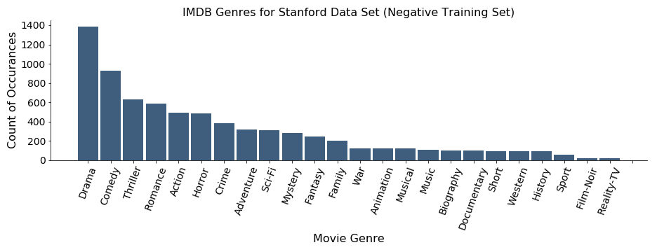
There are a lot of dramas and comedies in the dataset, some romance, action and sci-Fi movies and only a few Westerns, Documentaries and Sports-related films.

Movies in the dataset can also have multiple genres attached to them. For example, according to IMDB, Stanley & Iris is classified as both a drama and a romance.

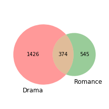IMDB-labeled movie genres overlap in a very intuitive way. For example, as shown to the left, a significant number of Romance movies are also Dramas. The converse is not as strong – i.e., there are a lot of drama movies that are not considered romances. This also seems intuitive – dramas can be much more than just romances.

We can visualize the relationships between co-occurances of different genres with a clustermap

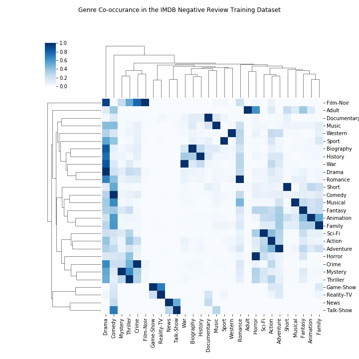
Once again the results are somewhat intuitive. The “Drama” genre co-occurs with many different smaller genres (strong co-occurances especially occur with “Sport” and “War”) while there are a few strong relationships to be seen (“News” and “Talk Show” for example).

We can use this data to help us design the proper classification problem.

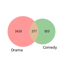From the bar graph above we know there is plenty of reviews for “Drama” and “Comedy” movies. We can also see that their co-occurance isn’t overwhelming, i.e., only 277 movies in the negative set are labeled both “Comedy” and “Drama”. This provides a good starting problem – how well can we train a classifier to detect if a movie is a “Comedy” or a “Drama”?

Building an NLP Classifier

For this exercise we are going to look at the performance of binary classifiers, i.e., how well a classifier labels a movie with a given genre. This aligns well with the dataset since a movie can have multiple labels. For example, “Die Hard” is both an Action and Thriller. A production-version design of this application could be a “bank” of binary classifiers, each one trying to determine if a given movie should be labeled with a specific genre.

To start lets consider two different classification approaches, a Convolutional Neural Net and a Logistic Regression classifier. We will compare performance on one genre and then extend to all of the genres in the IMDB dataset.

Dynamic Convolutional Neural Net

The implementation used for this analysis is taken from this great blog post, which in turn is an implementation of this algorithm. I recommend this post for a good primer on convolutional neural networks for NLP tasks.

The architecture of the network is shown below (image from Denny Britz ):

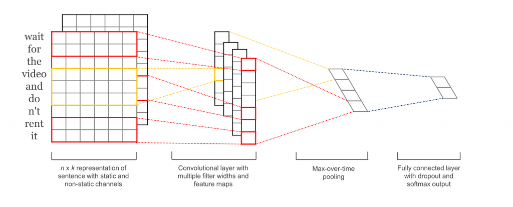
The input data is a word-embedding vector of the movie review. I used the Stanford GloVe dataset of word vectors. In this sense our DCNN model is a transfer learning model – we are taking the output of the pre-trained GloVe model and passing it through the DCNN.

After entering the neural net the data goes through a set of convolution, pooling, activation, folding, flattening and padding layers to ultimately produce a prediction vector for the genre-under-test.

Logistic Regression

The other model we will consider is a traditional logistic regression model. This classifier maps the output score of a fitted log regression curve and assigns a class to the data based on an optimal threshold.

The implementation used for this analysis is based on another nice blog post, this one by Zac Stewart. Our pipeline is pretty straight-forward:

pipeline = Pipeline([
    ('vect', CountVectorizer(ngram_range=(1, 3))),
    ('tf_idf', TfidfTransformer()),
    ('clf', LogisticRegression(C=0.39810717055349731,
                               class_weight=None)), ])

The first step in the pipeline vectorizes the comments into unigrams, bigrams and trigrams. Next, those vectors are tf-idf transformed, which weights the counts produced by the vectorizer by frequency within, and outside of the movie review. Lastly, the log regression model is built off the vectors. The penalty weight, C, was derived offline.

Performance Results

We are going to compare performance of the two approaches outlined above (the DCNN and Log Regression classifier) and then generalize to illustrate performance.

Performance Comparision (The Bakeoff)

Let’s start by looking at classifier performance for “Action” movies in the IMDB dataset. As discussed above, there are 25,000 movie reviews in the training folder as organized by Stanford, and 25,000 movie reviews in the test set. Of these, 4,414 and 4,302 of the reviews are for Action movies (respectively).

We fit both models to the training data and then apply the models to the test data. We can compare performance from several different perspectives.

The first comparison is to look at the different label scores that come out of the classifiers.

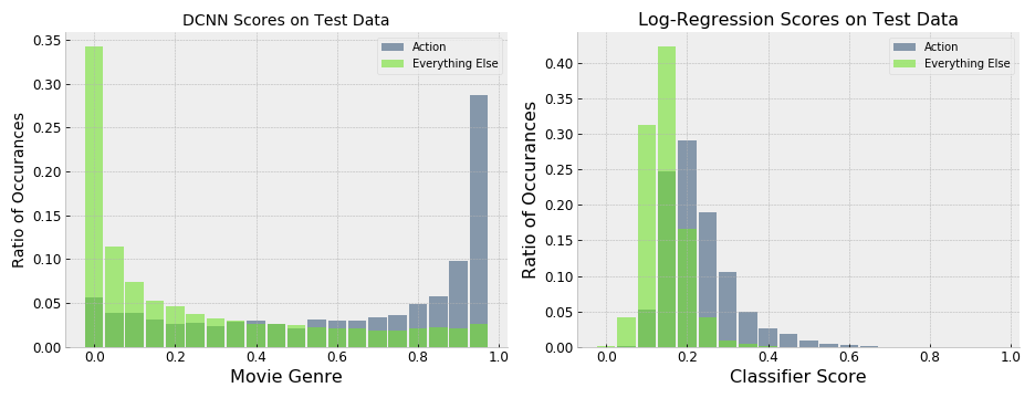
The classifiers distribute the genre scores much differently – you can see that the neural net scores primarily live on the poles of scoring region (i.e., are either 0 or 1) while the regression classifier distributes the scores primarily across the lower half of the scoring region.

A traditional next-step in evaluating classifier performance is to plot a Receiver-Operating-Curve (ROC) and measure the area under the curve. A ROC curve is generated by sweeping across a parameter of interest (in this case the threshold upon which a classifier score is used to determine the film to be an ‘Action’ movie) and measuring the resultant true and false positives that come from the classifier labels.

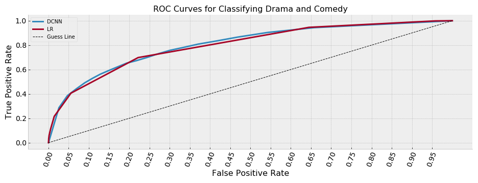
Interestingly, with respect to the ROC curves, the classifiers perform about the same ¹. The area-under-curve (AUC) for the two ROC curves is approximately the same. This also bears out if we report precision, recall and f1 for the different approaches (taken at the optimal f1 threshold for each classifier).

Measure	DCNN	Log Regression
Threshold	0.7	0.22
Precision	0.48	0.49
Recall	0.56	0.58
F1	0.52	0.53

Lastly, we can look at how many reviews the classifiers agree/disagree on.

	Total	Both Correct	DCNN Only	LR Only	Both Wrong
Action	4,302	1,983	432	511	1,376
Not-Action	20,428	16,509	1,303	1,325	1,291

It’s interesting that there so many reviews (nearly 25% of the Action movies) that the classifiers disagree on. Here’s just one example (the 1998 movie “Shepherd”. The DCNN correctly labeled it ‘Action’ while the LR classifier did not):

Shepherd (1998) If “B” movies, tired and corny scripts, and golf carts dressed up as some sort of futuristic mode of transport are your sort of entertainment, you’ll probably enjoy this. Otherwise, forget it. The topless newsreader, though completely irrelevant, did give a few seconds of amusement.

It’s easy to imagine a classifier getting tripped up by this review – there aren’t many clues it’s an Action movie.

Performance Across All Genres

Next Steps

1: I am far from a neural net expert and I’m not trying to suggest that a log regression classifier is equal to the DCNN. I didn’t even fully train the DCNN and am sure someone could tune it to have it outperform the regression approach.